Introduction to Embeddings and Semantic Search

When someone searches for “how to fry an egg” and your system returns results like “basic cooking techniques,” that’s semantic search. Semantic search “understands” the meaning of what you’re asking for and searches for related terms. There’s no exact word match, but there is semantic understanding. The technical piece that makes this possible is called an embedding, and in this post I’m going to explain how it works from the ground up: what a text vector is, why cosine similarity is the right metric, and how you build a complete pipeline in production.

From text to numbers: what is an embedding

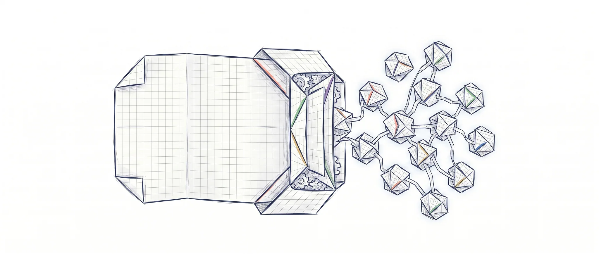
A language model can’t directly understand the word “cat” or “dog.” It needs to transform it into something it can understand. But it can’t do it any way — it needs to do it in a way that captures that these words are related in some way (they walk on four legs, they’re mammals, they’re alive…), and it needs to do it in a way that a computer can understand with math.

An embedding solves this: it transforms each piece of text into a vector of hundreds or thousands of numbers, trained so that texts with similar meaning produce similar vectors. “Cat” and “feline” end up close in that numerical space. “Cat” and “accounting” end up far apart.

The complete process has three steps: First, the text is divided into chunks or “tokens.” Tokens aren’t always complete words, but fragments of text with their own meaning.

The embedding model (a neural network trained on large sets of text) reads those tokens and produces a fixed-dimension vector. For OpenAI’s text-embedding-3-small tokenizer (AI model), that vector has 1536 dimensions. For text-embedding-3-large, it reaches 3072.

Each one of those 1536 numbers captures an aspect of the meaning of that text.

The analogy that works best for me: think of GPS coordinates. A geographic location is defined by latitude and longitude — two numbers that capture “where” that point is on the planet. An embedding does the same thing with meaning: it captures “where” that text is in semantic space, but instead of 2 dimensions, it uses 1536.

The vector space: where meaning transforms into vectors

Visualizing 1536 dimensions is impossible for the human brain. But if we compress that space to 2 or 3 dimensions (techniques like PCA or t-SNE do that), the pattern that emerges lets us see more clearly what embeddings consist of:

Programming terms cluster together. Cooking terms form another group (cluster). Sports terms form another. This distribution wasn’t specifically defined; it emerged from training the model on real human text. The model learned that “Python” and “debugging” appear in similar contexts, and that’s reflected in their vector position.

What this means for your searches: when a user types “bug in my code,” the vector of that query will fall close to “error in the application,” “uncaught exception,” “production failure” — even though none of those phrases share words with the original query.

Cosine similarity: the metric that lets us know when two texts are similar

You have two vectors. How do you measure how similar they are?

If we imagine the vector as an arrow pointing toward the meaning of that text, two vectors will be similar if they point in the same direction. We won’t worry about the exact point, just the direction.

To measure whether two vectors point in the same direction, we use cosine similarity. This is the mathematical calculation we use to know if two embeddings are similar.

Cosine similarity measures the angle between two vectors:

cos(θ) = (A · B) / (|A| × |B|)

The result ranges from -1 to 1. Two identical vectors have similarity 1.

Perpendicular vectors (unrelated) have similarity 0. Opposite vectors have similarity -1. In practice, with text embeddings, the values usually fall between 0 and 1 — texts are rarely semantically opposite in the strict sense.

Geometric intuition: two vectors pointing in the same direction are similar, regardless of whether one is longer than the other. It’s like comparing the orientation of two compasses, not the distance between them.

Practical applications: beyond search

Semantic search is the most visible use case — we compare one text against others to find similar ones — but embeddings open up a range of possibilities that goes well beyond that.

Semantic search: the user types a query, you convert it to an embedding, you search for the closest documents. It works even if the user uses different vocabulary than your documents. We’re searching by meaning, not by exact word match.

Recommendation systems: you convert each item (product, article, movie) into an embedding based on its description. To recommend, you search for items closest to the user’s history and interest description. You can generate this interest description with another model that interprets their behavior (what they’ve said they like, what they’ve searched for before, what they’ve visited…).

Semantic clustering: applying algorithms like “k-means” or similar to the embeddings of your documents. k-means looks for embeddings that are close together and groups them, so you can generate “idea clouds.” The clusters that emerge group content by similar topics without you having to define those topics manually. It’s useful for analyzing large volumes of user feedback or support tickets.

Anomaly detection: when most content is coherent, anomalous content (spam, off-topic content, duplicates with variations) produces vectors that end up isolated far from the main clusters. You can use embeddings to detect these anomalies.

Embeddings in production: vector databases

When you have thousands or millions of documents, comparing the query vector against each document one by one is unfeasible. You need specialized indexes that do approximate nearest neighbor (ANN) search in milliseconds.

The main options for vector databases:

Option	When to use it	Main advantage	Disadvantage
pgvector	You already have PostgreSQL, medium scale	No new infrastructure, normal SQL queries	Slower than dedicated high-scale solutions
Pinecone	You want managed, no ops	Zero infrastructure configuration	High cost at scale, vendor lock-in
ChromaDB	Local prototyping, development	Trivial installation, works in memory	Not suitable for production with real volume

About chunking: how you divide your documents before generating embeddings matters more than it seems. A 50-page document shouldn’t become a single embedding — you’d lose all granularity. But chunks that are too small lose context. In practice, chunks of 300-500 tokens with 50-100 token overlap is a reasonable starting point. The overlap between chunks ensures that ideas crossing a chunk boundary aren’t lost.

The embedding model also has a token limit. text-embedding-3-small accepts up to 8191 input tokens — text exceeding that limit is silently truncated if you don’t handle it.

The connection to RAG

If you’ve reached this point and think “this sounds like the foundation of question-answering systems over custom documents,” you’re right. Embeddings are the central piece of RAG (Retrieval-Augmented Generation): the pattern of retrieving relevant context before generating an answer with the LLM.

The complete RAG pipeline has more layers — more sophisticated chunking strategies, result re-ranking, handling of ambiguous queries, relevance evaluation. If you’re building a RAG system for production, the post Complete Enterprise RAG covers those layers in detail.

Common mistakes

Using embeddings for exact comparison

Embeddings measure semantic similarity, not identity. “Madrid is the capital of Spain” and “the Spanish capital is Madrid” will have high cosine similarity — and that’s correct. But if you need to detect whether two strings are exactly equal, a hash is faster, cheaper, and more precise. Embeddings are the wrong tool for that job.

Not normalizing vectors before storing them

Some models return already-normalized vectors (magnitude = 1). Others don’t. If you mix vectors from different sources or model versions without normalizing, cosine similarity stops being a fair comparison. Always normalize before persisting — it’s a cheap operation that prevents hard-to-detect bugs.

Chunks that are too large

I saw this error in a project where someone converted entire documentation pages into a single embedding. The result: the vector averaged too many distinct concepts and the search always returned the longest pages, not the most relevant ones. One embedding per paragraph, with overlap between consecutive paragraphs, solves this.

Generating embeddings at query time for static documents

If you have 100,000 documents and re-embed them on every search, your latency will be unacceptable and so will your API bill. Document embeddings are precomputed and stored. Only the query embedding is generated in real time.

Changing the embedding model without re-indexing

The vectors from text-embedding-3-small and text-embedding-3-large live in different spaces — they’re not comparable to each other. If you migrate to a new model, you need to re-generate all the embeddings in your index. Always keep track of which model generated which vector.

Implementation checklist

• The embedding model is pinned with explicit version (not “latest”)

• Documents are divided into chunks of 300-500 tokens with 50-100 token overlap

• Vectors are normalized before being stored in the database

• Document embeddings are precomputed offline, not at query time

• The model that generated each vector is recorded along with the vector

• Cosine similarity (not Euclidean distance) is used to compare vectors

• Chunks exceeding the model’s token limit are detected and handled before calling the API

• There’s a defined strategy for re-indexing when switching models

Frequently Asked Questions

How many dimensions does an embedding need to be useful?

It depends on the task. For standard semantic search, 384 dimensions (models like all-MiniLM-L6-v2) work well and are more efficient in storage. OpenAI’s models with 1536 or 3072 dimensions capture finer nuances and generally give better results on complex tasks, but the quality jump doesn’t always justify the extra cost. The way to know is to measure on your actual data.

What’s the difference between word embeddings (Word2Vec) and sentence embeddings?

Word2Vec generates one vector per word, always the same regardless of context. “Bank” (furniture) and “bank” (financial) have the same vector. Modern sentence embedding models like OpenAI’s are contextual: the representation of a word depends on the surrounding words. This makes them much more precise for real semantic search.

Can I use embeddings without a vector database?

Yes, and it makes sense to do so in early stages. If you have fewer than 10,000 documents, you can store vectors in an in-memory array or a JSON file and calculate cosine similarity with NumPy or plain JavaScript. The example code in this post works that way. The vector database becomes necessary when volume grows or when you need combined filters (similarity + metadata).

Do embeddings capture language?

Multilingual models like OpenAI’s text-embedding-3-small are trained on multiple languages and can compare texts across languages. A query in English can return relevant documents in Spanish. Monolingual models are more precise within their language, but fail at cross-language comparisons. For applications in Spanish with Spanish-speaking users, a quality multilingual model is usually sufficient.

When to use semantic search versus keyword search (BM25)?

They’re not mutually exclusive. Keyword search (BM25, Elasticsearch) is very precise when the user knows exactly what term to search for and that term is in the documents. Semantic search shines when the user describes a concept in their own words or when documents use different vocabulary than the query. The most robust pattern in production is hybrid search: run both in parallel and merge results with an algorithm like Reciprocal Rank Fusion (RRF).